Learn how to detect objects with deep learning and track their movement over time.
Author
Adrien Vandekerckhove
Published
February 28, 2023
Introduction
If you want to directly see the results, click here. Otherwise, I will explain the steps and ideas developed in this article as I implement them.
The goal here is to showcase what is possible with computer vision and recent deep learning techniques. The one we will study here is called multi-object tracking (MOT). We will see that MOT is a direct upgrade from object detection.
With object detection, the model is trained to predict a label and a bounding box to some objects in the scene. One limitation of that approach is that it is not suited for studying the behavior of those objects over time since there is no relation between objects from one frame to another. That’s when multi-object tracking comes in handy. For each object in the scene, it will first be detected by a detection model (Yolov5 for example) and then associated an id to keep track of it between each frame. This approach is quite powerful if a workflow requires an understanding of the movement of objects (take self driving-cars as an example).
For the sake of simplicity in this demo, we will use MOT to detect and track people in a shopping center. The scene is kept simple to showcase the main ideas with MOT.
Let’s outline the general approach taken here :
Find a source video
Apply an MOT model to the video
Save the results of MOT
Transform the results
Analyze the results
Load them nicely in a video
Let’s now outline the tools and methods for each point :
We simply save the results as a csv file, if you know that you will process lots of data, parquet is better suited
We will extract a bit more information from the bboxes like speed on the x and y-axis.
Once we have all the raw results from the tracking and the new features, we can do some exploratory analysis of the data.
Finally, we will reconstruct a video that adds new information about the scene with OpenCV
Note: Deep Sort isn’t the newest MOT model but still has good accuracy and is enough for our use case. For more information on the state of the art in MOT, take a look at Papers with Code for the MOT20 benchmark
Note
Deep Sort isn’t the newest MOT model but still has good accuracy and is enough for our use case. For more information on the state of the art in MOT, take a look at Papers with Code for the MOT20 benchmark
Finding a source video
Importing the necessary libraries
import matplotlib.pyplot as pltimport seaborn as snsimport pandas as pdimport numpy as npimport mmcvimport cv2from mmtrack.apis import inference_mot, init_modelfrom dataclasses import dataclass, asdictfrom shapely import Polygon, Pointfrom IPython.display import Videofrom pathlib import Pathfrom tqdm import tqdm
Here is the video we will be working with :
Video("people.mp4")
Apply MOT on the video
Once mmtracking is installed, it is easy to run inference with models supported by the library. The two main methods are init_model for loading a model and inference_mot to run inference from a multi object tracking model. You can then call the show_result to get a new frame where the bboxes are drawn.
def track_video(input_video, out_path, out_video_name, config=MOT_CONFIG): imgs = mmcv.VideoReader(input_video) mot_model = init_model(config, device='cuda:0') Path(out_path).mkdir(parents=True, exist_ok=True) results = []for i, img inenumerate(imgs):if i %100==0:print(f'processing frame {i}') result = inference_mot(mot_model, img, frame_id=i) results.append(result) mot_model.show_result( img, result, show=False, wait_time=int(1000./ imgs.fps), out_file=f'{out_path}/{i:06d}.jpg')print(f'\n making the output video at {out_path} with a FPS of {imgs.fps}') mmcv.frames2video(out_path, out_video_name, fps=imgs.fps, fourcc='FMP4')return results
We can now call the previous function with the input video we chose, the folder that will contain the new frames and the name for the newly constructed video.
Like before, we can display the video with from IPython.display import Video.
Video("tracking.mp4")
We can see that Deep Sort performs quite well in this specific environment. We need to keep in mind that the camera angle is quite good and that there nothing is cluttering the view of the camera. Those factors play a big role in the accuracy of the model. Still, some people may sometimes be mislabeled or simply won’t be detected. Those things should be handled with precaution if one wants to use MOT in production.
Save the results of MOT
To simplify our conversion of the results of Deep Sort to a pandas Dataframe, we will use a dataclass. This makes it easier to see what attributes we will be working with.
@dataclassclass Person: time_step: intid: int xmin: float ymin: float xmax: float ymax: float score: float@propertydef centroid_x(self):returnself.xmin + (self.xmax -self.xmin) /2@propertydef centroid_y(self):returnself.ymin + (self.ymax -self.ymin) /2def__lt__(self, o):returnself.id< o.iddef asdict(self): data = asdict(self) data["centroid_x"] =self.centroid_x data["centroid_y"] =self.centroid_yreturn data@classmethoddef df_from_tracking_results(cls, results) -> pd.DataFrame: data = []for i, result inenumerate(results):for track_bboxes in result["track_bboxes"]:for bbox in track_bboxes: person = Person(i, *bbox) person.id=int(person.id) data.append(person)return pd.json_normalize(obj.asdict() for obj in data)
We can now simply construct a dataframe for any MOT model results from mmtracking with our dataclass.
In this section, we will load and apply some simple transformations to our csv file to extract more interesting properties. First, we will look at the results contained in our csv file.
I said earlier that one limitation of object detection is that we cannot study the behavior of objects in time because we cannot reidentify an object that appeared previously. We will see here that by removing this limitation, we can have a richer insight of the data. I will demonstrate it by using the speed variable.
As you can see, for each person, at each frame, we can estimate the speed. Note that the speed here is expressed as px/frame and not in m/s. For accurate speed prediction, we would need a camera that predicts the depth of each pixel. Without it, we can only make gross estimations based on some reference points.
We will come back later to the speed variables when we will study the behavior of people over time.
Region detection
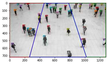
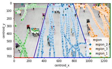
Another thing that we can do is to define specific regions on the camera/video. We can then detect people in those zones and if they are crossing one of them. Here, we will work with 3 regions I handpicked.
In practice it, could be used for prevention by detecting dangerous events like a car stuck on train tracks and sending an alert to the train driver ahead of time.
Outliers are not easy to handle. Here they arise from the Deep Sort model’s bad predictions. This means that we could get someone that is located in the top left corner of the camera and goes to the bottom right corner in one frame. The way outliers are treated should be dependent on the task being done. Here, we simply want to analyze the data and reconstruct a new video that takes the regions into account. That is why we will use simple techniques to remove them.
Position incoherence
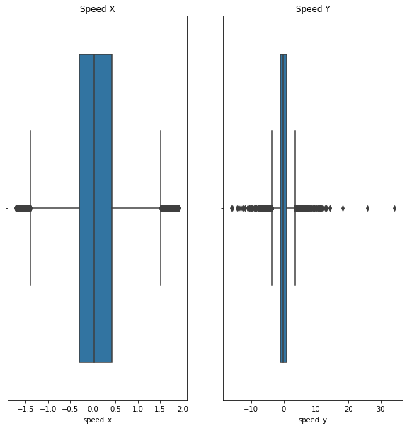
As I said, it is possible that the same person is detected at two locations that don’t make sense between each frame. This can be seen with a box plot of the speed samples.
# Show the violin plots of the features that interest usfig, ax = plt.subplots(1, 2, figsize=(10, 10))sns.boxplot(data=df, x="speed_x", ax=ax[0])sns.boxplot(data=df, x="speed_y", ax=ax[1])# Add titles to the plotsax[0].set_title("Speed X")ax[1].set_title("Speed Y")# Set limits to the x-axisax[0].set(xlim=(-100, 100))ax[1].set(xlim=(-100, 100))
[(-100.0, 100.0)]
As you can see, there are a lot of outliers at values that don’t seem to be possible. The outliers seen on the boxplot can be detected using the interquartile range (IQR). We will use that method to remove them.
The plots will now look a lot nicer without the extreme outliers.
# Show the violin plots of the features that interest usfig, ax = plt.subplots(1, 2, figsize=(10, 10))sns.boxplot(data=df, x="speed_x", ax=ax[0])sns.boxplot(data=df, x="speed_y", ax=ax[1])# Add titles to the plotsax[0].set_title("Speed X")ax[1].set_title("Speed Y")
Text(0.5, 1.0, 'Speed Y')
Missing values
We will also drop missing values
df = df.dropna()
Analyze the results
Now that we have a nice dataframe, we can look at the interesting part. Visualizing behavior over time. On our input video, we can see many people walking in a shopping center, we can also see that some of them are standing. We could then ask ourselves an interesting question: “What is the default behavior of the people seen on the camera, standing or walking ?” This is what we will answer in this section.
The first step is to create new columns that indicate the time associated with the frame in seconds.
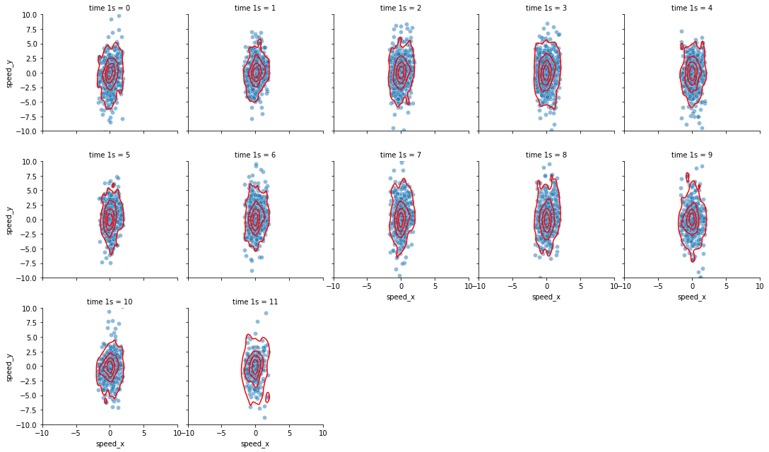
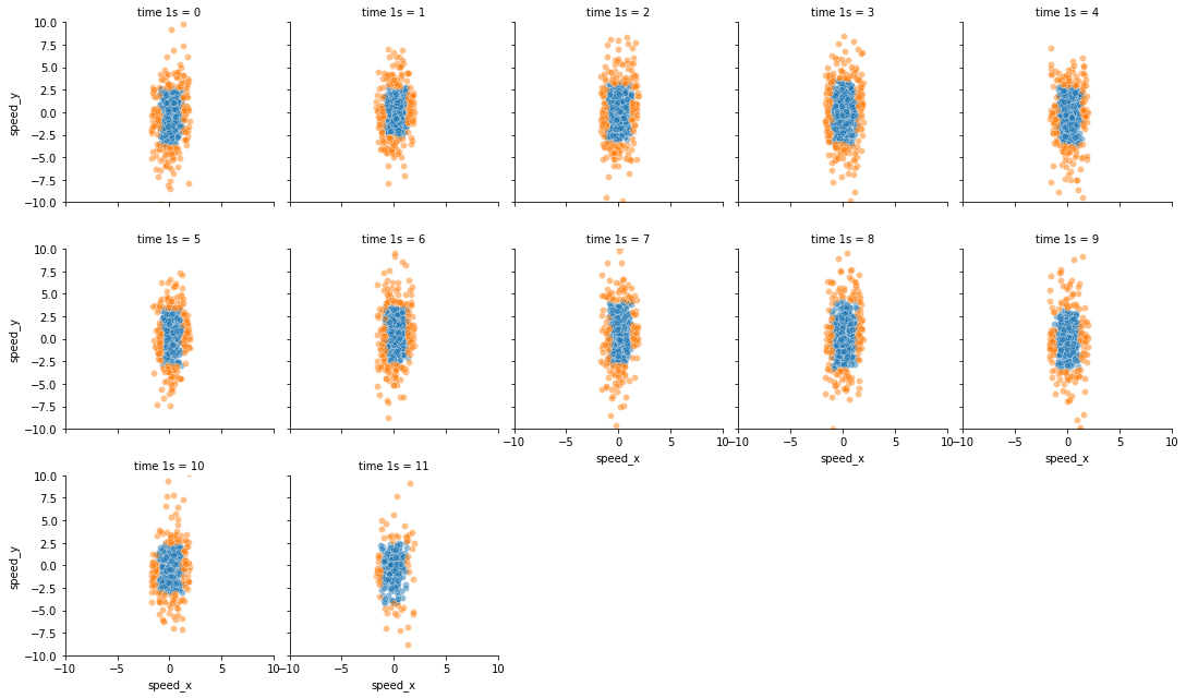
Now, all we need to do is to estimate the distributions of the speed of the x and y axis and look at the samples at the heads and tails of those distributions. We can sum up that idea quite simply by using seaborn to display the samples and the kernel density estimations over speed_x and speed_y. By default, the kde_plot uses the 5th and 95th percentile to draw the outermost contour line.
You can easily see on those plots that people are more likely to move fast from top to bottom on the camera than left to right. We can also answer our first question. Whilst there are people standing (the first contour line encapsulates the values close to zero for speed_x and speed_y) there are many more who are moving slowly or faster (the other four contour lines).
To be sure that we didn’t make any mistakes when selecting the outliers, we can plot our samples with a color for the outliers and another one for the rest of the data points.
We can see that for each point that was outside the kernel density estimation, we correctly identified the point as an outlier.
This concludes this section. I showed how one can try and extract new information from a video by linking the objects in each frame thanks to MOT and we were able to extract insight that would not have been possible with simple object detection.
Load the results nicely in a video
In this section, we will use OpenCV to create a new video that takes the regions into account.
Similarly to the way we used a dataclass to create our dataframe, we will use a dataclass to help us draw the needed information on the screen.
@dataclassclass Person: time_step: intid: int xmin: int ymin: int xmax: int ymax: int score: float centroid_x: int centroid_y: int speed_x: int speed_y: int d_time_step: int speed: int region: str time_1s: int time_5s: int time_20s: int outlier_speed_x: bool outlier_speed_y: bool outlier_speed: booldef__le__(self, other):return (self.time_step, self.id) <= (other.time_step, other.id)@classmethoddef from_dataframe(cls, df):return [cls(*row) for row in df.itertuples(index=False)]def _draw_bbox(self, img): color = (0, 0, 0)ifself.region =="region_1": color = COLOR_1elifself.region =="region_2": color = COLOR_2elifself.region =="region_3": color = COLOR_3 cv2.rectangle(img, (int(self.xmin), int(self.ymin)), (int(self.xmax), int(self.ymax)), color, 1)def _draw_text(self, img, text, color=(0, 0, 0), offset=(0, 0)): offset_x, offset_y = offset cv2.putText(img, text, (int(self.xmin) + offset_x, int(self.ymin) + offset_y), cv2.FONT_HERSHEY_SIMPLEX, 0.25, color, 1, cv2.LINE_AA)def _draw_labels(self, img, color=(0, 0, 0)):self._draw_text(img, f"ID:{self.id}", color, (0, -10))self._draw_text(img, f"SCORE:{self.score:.2f}", color, (0, -20))def draw(self, img):self._draw_bbox(img)self._draw_labels(img, COLOR_4)
Here we are constructing a dictionary with the time_step as the key and that contains a list with all the people appearing at that time_step
persons = Person.from_dataframe(df)dic = {}outliers = {}for person in persons:if person.time_step notin dic: dic[person.time_step] = [] dic[person.time_step].append(person)
We can now use OpenCV to make a new video that we will call output.mp4
out = cv2.VideoWriter('output.mp4',cv2.VideoWriter_fourcc(*"FMP4"), 30, (1280,720))cap = cv2.VideoCapture("people.mp4")counts = df.groupby(["time_step", "region"])["region"].count()total_frames =int(cap.get(cv2.CAP_PROP_FRAME_COUNT))for i in tqdm(range(total_frames)): _, image = cap.read()# Initially, no one is detectedif i notin dic: out.write(image)continue# Drawing the regions cv2.polylines(image, [np.array(region1.exterior.coords).astype(np.int32)], True, COLOR_1, 2) cv2.polylines(image, [np.array(region3.exterior.coords).astype(np.int32)], True, COLOR_3, 2) cv2.polylines(image, [np.array(region2.exterior.coords).astype(np.int32)], True, COLOR_2, 2)# Counting the number of people in each region count1 = counts[(i, "region_1")] count2 = counts[(i, "region_2")] count3 = counts[(i, "region_3")]# Drawing the number of people in each region cv2.putText(image, f"Region 1: {count1}", (10, 20), cv2.FONT_HERSHEY_SIMPLEX, 0.5, COLOR_1, 1, cv2.LINE_AA) cv2.putText(image, f"Region 2: {count2}", (10, 40), cv2.FONT_HERSHEY_SIMPLEX, 0.5, COLOR_2, 1, cv2.LINE_AA) cv2.putText(image, f"Region 3: {count3}", (10, 60), cv2.FONT_HERSHEY_SIMPLEX, 0.5, COLOR_3, 1, cv2.LINE_AA)# Drawing the bounding boxes and labelsfor person in dic[i]: person.draw(image) out.write(image)cap.release()out.release()
100%|██████████| 341/341 [00:05<00:00, 62.18it/s]
Finally, we will display the results of our work.
Here is the video we took as input.
Video("people.mp4")
Here is the video we got by applying Deep Sort.
Video("tracking.mp4")
And here is the final video we got by combining Deep Sort and adding regions to the scene.
Video("output.mp4")
Conclusion
This concludes what I wanted to show with this demonstration. We touched upon many topics in Computer Vision and Machine Learning and applied them to answer some interesting questions we can ask ourselves about the data.
As I mentioned earlier, the models are not limited to people. You can track any kind of object. The most common ones will be accessible via pre-trained models. But you can also fine-tune those models or retrain parts of them to get what you want out of multi-object tracking.
If you follow the methodology presented here, you will be able to construct your own solutions to problems that involve computer vision systems.